Advanced R for Econometricians

Advanced R for EconometriciansImproving PerformanceMartin C. Arnold1 / 55

Improving Performance

# packages needed
library(tidyverse) # for bench package
library(parallel)
library(MonteCarlo)

We should forget about small efficiencies, say about 97% of the time: premature optimisation is the root of all evil. Yet we should not pass up our opportunities in that critical 3%. A good programmer will not be lulled into complacency by such reasoning, he will be wise to look carefully at the critical code; but only after that code has been identified. — Donald Knuth

2 / 55

Improving Performance — Overview

Once profiling has revealed a bottleneck, we need to make it faster. In the following we will discuss some techniques that are broadly useful:

Look for existing solutions.

Searching google can save you lots of time. The benefit of finding a faster (but possibly suboptimal) solution on your own may be small.
Do as little as possible. Be precise.

Using optimized functions tailored for specific tasks often makes a big difference.
Vectorise your code.

This often relates to avoiding loops and the associated inefficiencies.
Parallelise (if possible).

Using multiple CPU cores in parallel is enormously helpful when the computation involves a large number of tasks that may be solved independently.

3 / 55

1. Look for Existing Solutions

There's a good chance that someone has already tackled the same problem.

Find out if there is a Cran Task View related to your problem and search the packages listed there
Limit your search to packages that depend on the Rcpp package (and thus likely implement high-performant C++ code). This is easily done by checking reverse dependencies of Rcpp.
Check if a question related to your problem has been asked on stackoverflow. Narrow the search by using suitable tags, e.g., [r], [performance].
Google. For R-related results, use rseek.

Record all solutions that you find not just those that immediately appear to be faster!

Some solutions might be initially slower but are are easier to optimize and thus end up being faster.
Sometimes combining the fastest parts from different approaches is helpful.

4 / 55

Improving Performance — Golden Rule

Before we continue, we introduce a rule we have already followed implicitly: the golden rule of R programming:

Access the underlying C/FORTRAN routines as quickly as possible; the fewer functions calls required to achieve this, the better.

(Lovelace and Gillespie, 2016)

The techniques discussed next follow this paradigm. If this is not enough, we still may rewrite (some of) the code in C++ using the Rcpp package (discussed in the next chapter).

5 / 55

2. Do as Little as Possible

If you cannot find existing solutions, start by reducing your code to the bare essentials.

Exercise: coercion of inputs / robustness checks

X <- matrix(1:1000, ncol = 10)
Y <- as.data.frame(X)

Which approach is faster and why?

apply(X, 1, sum)
apply(Y, 1, sum)

6 / 55

2. Do as Little as Possible

A function is faster if it has less to do — obvious but often neglected!

Use functions tailored to specific input and output types / specific problems!

Exercise: coercion of inputs / robustness checks — ctd.

Which approach is faster and why?

rowSums(X)
apply(X, 1, sum)

7 / 55

2. Do as Little as Possible

Exercise: searching a vector

What is the fastest way to check if 10 is an element of 1:100?

8 / 55

2. Do as Little as Possible

Exercise: Linear Regression — computation of $S E (\hat{β})$

Which approach is faster and why? Name disadvantages of the fastest one.

set.seed(1)
X <- matrix(rnorm(100), ncol = 1)
Y <- X + rnorm(100)
a <- function() {
  coefficients(summary(lm(Y ~ X - 1)))[1, 2]  
}
b <- function() {
  fit <- lm.fit(X, Y)
  c(
    sqrt(1/(length(X)-1) * sum(fit$residuals^2) * solve(t(X) %*% X))
    )
}

9 / 55

2. Do as Little as Possible

Be as explicit as possible.

Example: method dispatch takes time

x <- runif(1e2)
bench::mark(
  mean(x),
  mean.default(x)
)

## # A tibble: 2 x 6
##   expression           min   median `itr/sec` mem_alloc `gc/sec`
##   <bch:expr>      <bch:tm> <bch:tm>     <dbl> <bch:byt>    <dbl>
## 1 mean(x)           2.64µs   3.07µs   297320.    22.7KB      0  
## 2 mean.default(x)   1.13µs   1.35µs   659992.        0B     66.0

10 / 55

2. Do as Little as Possible

Benchmark against alternatives that rely on primitive functions.

Example: primitives are faster

bench::mark(
  mean.default(x),
  sum(x)/length(x)
)

## # A tibble: 2 x 6
##   expression            min   median `itr/sec` mem_alloc `gc/sec`
##   <bch:expr>       <bch:tm> <bch:tm>     <dbl> <bch:byt>    <dbl>
## 1 mean.default(x)    1.15µs   1.38µs   658724.        0B        0
## 2 sum(x)/length(x)    432ns    526ns  1637111.        0B        0

11 / 55

2. Do as Little as Possible — Exercises

Can you come up with an even faster implementation of b() in the linear regression example?

What’s the difference between rowSums() and .rowSums()?

rowSums2() is an alternative implementation of rowSums(). Is it faster for the input df? Why?

rowSums2 <- function(df) {
  out <- df[[1L]]
  if (ncol(df) == 1) return(out)
    for (i in 2:ncol(df)) {
      out <- out + df[[i]]
    }
  out
}
df <- as.data.frame(
  replicate(1e3, sample(100, 1e4, replace = TRUE))
)

12 / 55

2. Do as Little as Possible — Case Study

Imagine you want to compute the bootstrap distribution of a sample correlation coefficient using cor_df() and the data in the example below.

Given that you want to run this many times, how can you make this code faster?

n <- 1e6
df <- data.frame(a = rnorm(n), b = rnorm(n))
cor_df <- function(df, n) {
  i <- sample(seq(n), n, replace = TRUE)
  cor(df[i, , drop = FALSE])[2, 1]
}

13 / 55

3. Vectorise your code

What is vectorisation?

Vectorisation is the process of converting an algorithm from operating on a single value at a time to operating on a set of values (like a vector) at one time.
It makes problems simpler: code that operates on vectors instead of single entries of an array is often less complex to write.

Why is it efficient?

(on the lowest level where functions map closely to processor instructions)

Your computer is designed to run vectorised operations: a vectorised function may run multiple operations from a single instruction which is faster than sending individual instructions for each operation.

14 / 55

3. Vectorise your code

Why is vectorisation efficient? — ctd.

Many languages (including R) work on arrays that are stored in the memory in column-major order.

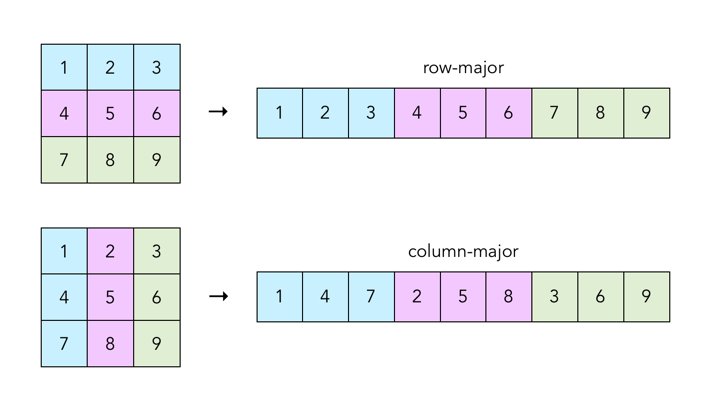
Disregarding these patterns by writing code which operates on $1 \times 1$ vectors thus means 'fighting the language'.

15 / 55

3. Vectorise your code

Why is vectorisation efficient? — ctd.

Example: vector addition

$(\begin{matrix} 1 \\ 2 \\ 3 \end{matrix}) + (\begin{matrix} 4 \\ 5 \\ 6 \end{matrix}) = (\begin{matrix} 5 \\ 7 \\ 9 \end{matrix})$

Slow: three instructions, three operations
- add $1$ and $4$
- add $2$ and $5$
- add $3$ and $6$
Fast: one instruction, one vectorised operation:
- add ${(\begin{matrix} 1 2 3 \end{matrix})}^{'}$ and ${(\begin{matrix} 4 5 6 \end{matrix})}^{'}$
- The three additions are effectively done in parallel.

16 / 55

Aagain, less related to R itself but to what the CPU does.

3. Vectorise your code

What does it mean to write 'vectorised' code in R?

Remember that there are no 'real' scalars in R. Everything that looks like a scalar is actually a $1 \times 1$ vector.

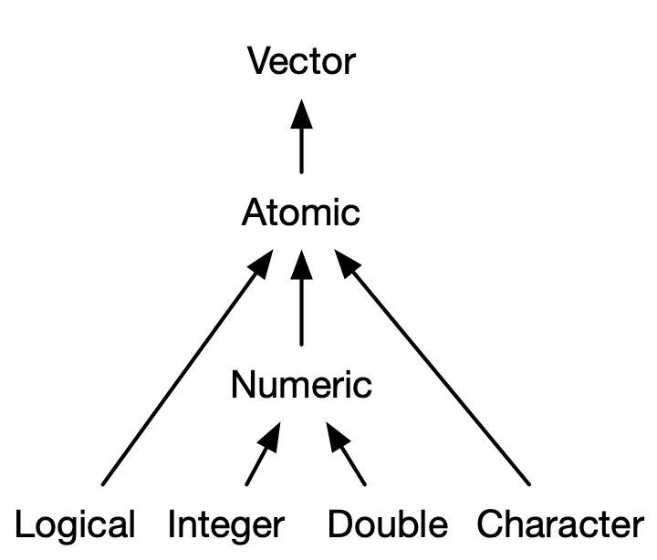
# otherwise this shouldn't work:
1[1]

## [1] 1

Thus 'scalar' operations work on vector elements which is (often) needlessly cumbersome.

17 / 55

3. Vectorise your code

What does it mean to write 'vectorised' code in R?

By 'vectorised' we mean that the function works on vectors, i.e., performs vector arithmetic and calls functions which work on vectors.

Example: scalar vs. vectorised computation of euclidean norm

L2_scalar <- function(x) {
  out <- numeric(1)
  for(i in 1:length(x)) {
    out <- x[i] * x[i] + out 
  }
  return(sqrt(out))
}

L2_vec <- function(x) {
 return(
   sqrt(
     sum(x * x)
     )
   )
}

18 / 55

3. Vectorise your code

What does it mean to write 'vectorised' code in R?

By 'vectorised' we mean that the function works on vectors, i.e., performs vector arithmetic and calls functions which work on vectors.

Example: scalar vs. vectorised computation of euclidean norm

bench::mark(
  L2_scalar(1:1e4),
  L2_vec(1:1e4)
)

## # A tibble: 2 x 6
##   expression              min   median `itr/sec` mem_alloc `gc/sec`
##   <bch:expr>         <bch:tm> <bch:tm>     <dbl> <bch:byt>    <dbl>
## 1 L2_scalar(1:10000)  713.1µs  775.8µs     1236.    4.11MB      0  
## 2 L2_vec(1:10000)      40.3µs   73.1µs    12708.   78.22KB     16.9

19 / 55

3. Vectorise your code — Some Principles

Do not torture the interpreter

Vectorisation reduces the amount of intepreting R has to do: Validating that x <- 1L and y <- 1:100L are of type integer is equally expensive. Checking that each element of y is an integer is not!
Use functions from base R that work on vectors

Vectorisation may avoid loops in R. Loops in many 'vectorised' R functions are carried out in C and thus are much faster.

The following functions are prominent examples:

rowSums(), colSums(), rowMeans(), colMeans(), cumsum(), diff()
Use matrix algebra

Most matrix operations that involve loops are executed by highly optimized external Fortran and C libraries. See, e.g., BLAS.

20 / 55

3. Vectorise your code

Are for() loops slower than *apply()?

for() loops have the reputation of being slow(er than *apply()). This is widespread wisdom and not generally true:

for() is not slow if we iterate over data and apply a (non-vectorised) function. Execution time is comparable to *apply().
Loops are often used in an inefficient manner:

Growing an object and improper initialisation means overhead due to growing / copying in every iteration.

Getting used to *apply() is a good practice as it prevents us from doing silly stuff like the above.

What if I need to use for / how to properly write a for loop?

Allocate the required storage before the loop and fill the object!

21 / 55

3. Vectorise your code

Example: avoid growing objects

22 / 55

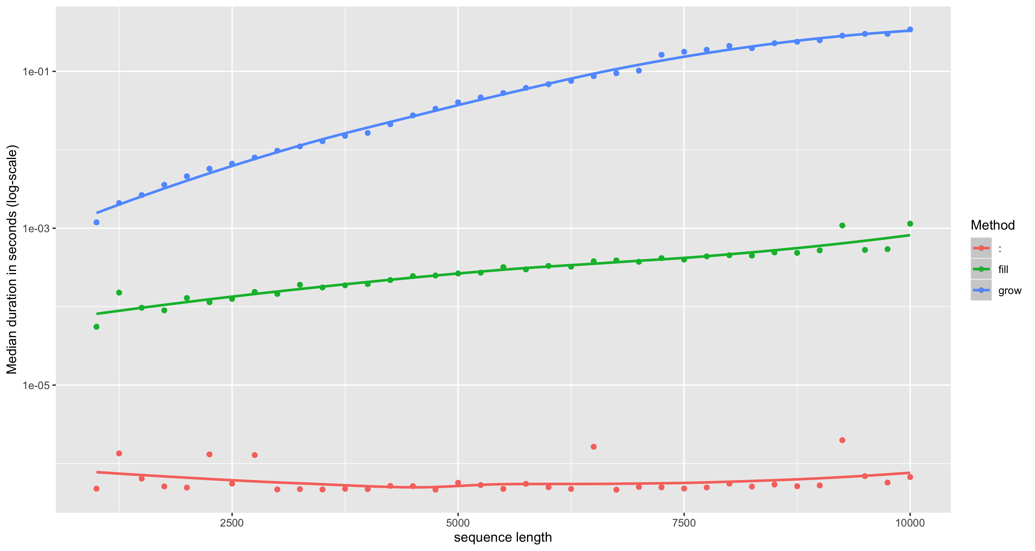
3. Vectorise your code

Example: good and bad `for()` loops

# Bad: c()/cbind()/rbind()
rw_bad <- function(N) {
  set.seed(1)
  out <- rnorm(1)
  for(i in 2:N) {
   out <- c(out, 
            out[i-1] + rnorm(1))
  }
  return(out)
}

23 / 55

3. Vectorise your code

Example: good and bad `for()` loops

# Good: proper initialisation/iteration
rw_good <- function(N) {
  set.seed(1)
  out <- vector("double", N)
  out[1] <- rnorm(1)
  for(i in 2:N) {
   out[i] <- rnorm(1) + out[i-1]
  }
  return(out)
}

24 / 55

3. Vectorise your code

Example: good and bad `for()` loops

bench::mark(rw_good(1e4), 
            rw_bad(1e4))

## # A tibble: 2 x 6
##   expression          min   median `itr/sec` mem_alloc `gc/sec`
##   <bch:expr>     <bch:tm> <bch:tm>     <dbl> <bch:byt>    <dbl>
## 1 rw_good(10000)   15.2ms   22.6ms     39.3     24.8MB     21.6
## 2 rw_bad(10000)     346ms  351.5ms      2.85   406.3MB     27.0

25 / 55

3. Vectorise your code

Are for() loops slower than the *apply() functions?

Example: `for()` vs. `apply()`

X <- matrix(rnorm(1e4), ncol = 1e4)
colmax <- function(x) {
  out <- numeric(ncol(x))
  for(j in 1:ncol(x)) {
    out[j] <- max(x[,j])
  }
  return(out)
}

26 / 55

3. Vectorise your code

Are for() loops slower than the *apply() functions?

Example: `for()` vs. `apply()` — ctd.

bench::mark(
  colmax(X),
  apply(X, 2, max)
)

## # A tibble: 2 x 6
##   expression            min   median `itr/sec` mem_alloc `gc/sec`
##   <bch:expr>       <bch:tm> <bch:tm>     <dbl> <bch:byt>    <dbl>
## 1 colmax(X)          5.75ms   6.37ms     156.     4.34MB     55.0
## 2 apply(X, 2, max)   9.05ms  10.27ms      96.6  312.73KB     55.2

27 / 55

3. Vectorise your code — Exercises

Compare the speed of apply(X, 1, sum) with the vectorised rowSums(X) for varying sizes of the square matrix X using bench::mark(). Consider the dimensions 1, 1e1, 1e2, 1e3, 0.5e4 and 1e5. Visualize the results using a violin plot.
(a) How can you vectorise the computation of a weighted sum?

(b) How can you use crossprod() to compute that same sum?

(c) Compare performance of the approaches in (a) and (b)
Find an approach to compute column maxima of a numeric matrix X using a *apply()-function which outperforms apply(X, 2, max).

28 / 55

3. Vectorise your code — Case Study

Case Study: Monte Carlo Integration

Suppose you are interested in computing $A = \int_{0}^{1} x^{2} d x$ using Monte Carlo (MC) integration. Consider the following algorithm which operates on $1 \times 1$ vectors in a for() loop:

initialize counts
for i in 1:N

Generate $U_{i} \sim i . i . d . U (0, 1); i = 1, 2$ .

If $U_{2} < U_{1}^{2}$ , then counts = counts + 1
end for
Estimate $A$ by counts/N

29 / 55

3. Vectorise your code — Case Study

Case Study: Monte Carlo Integration

(a) Implement the algorithm in a function A_loop(N). A should use a loop to compute the MC estimate of $A$ with N MC iterations.

(b) Estimate $A$ using A_loop(N) with 5e5 MC iterations.
(a) Define a function A_vec(N) which implements the MC algorithm using a vectorised approach.

(b) Compare A_vec(N) and A_loop(N) in a microbenchmark for N = 5e5 iterations.

(c) How does the difference in performance relate to N?

30 / 55

4. Parallelisation — FAQs

What is parallelisation?

In the simplest sense, parallelisation means the simultaneous use of multiple hardware resources for solving a computational problem.
In the following we refer to parallelisation as the distribution of computing tasks over several CPUs in a shared memory system (a system where multiple CPUs access the same memory).

Does R perform parallelisation by default?

No. The 'stock' R version on CRAN is a single-threaded program, i.e., R does not benefit from modern multi-threaded CPUs, multiple cores let alone multiple CPUs.

31 / 55

4. Parallelisation — FAQs

Is it complicated to parallelise code?

In general, yes. Fortunately, there are R packages for the most common platforms that do the work for us. These packages facilitate the process substantially.
In most cases, we don't even have to adjust our code in order for it to be executable in parallel.

Which tasks can be done in parallel?

In principle, all operations that can be executed independently.
Parallel computing is often used in MC simulations which require computation of a large number of homogeneous and independent tasks.

Is parallelisation always faster than 'serial' computation?

No. The cost of managing the computations (the overhead) may offset or even surpass time savings gained by parallel computation. This occurs, e.g., when a small number of simple tasks is solved in parallel. We will discuss an example.

32 / 55

4. Parallelisation — the `parallel` package

The parallel package (comes with base R) is a good starting point for parallel computing.

# detect numer of cores (including logical cores)
library(parallel)
detectCores()

## [1] 8

The notebook used to run this script has a 2,3 GHz Intel Core i5 processor with 4 physical CPUs and supports hyper-threading, i.e., each CPU has 2 logical cores.

# detect numer of physical cores
detectCores(logical = F)

## [1] 4

Note that the behavior of detectCores() is platform specific and not always reliable, see ?detectCores().

33 / 55

4. Parallelisation - `parallel::mclapply()`

Example: send them cores to sleep (on MacOS)

r <- mclapply(1:8, function(i) Sys.sleep(20), mc.cores = 8)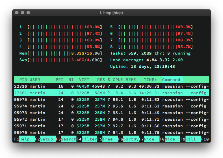

34 / 55

4. Parallelisation - `parallel::mclapply()`

Example: send them cores to sleep (on MacOS) — ctd.

What happened?

The R session (the main Process) opened 8 sub-processes, so-called forks (labeled rsession in the activity monitor)
The forks operate independently from the main process (but they 'know' about each other). Each fork operates on a separate core.
mclapply() passes a call of function(i) Sys.sleep(20) to each fork. Computation (or rather doing nothing for 20 seconds) now proceeds in parallel.
After 20 seconds the results are gathered in r and all forks are killed. Note that r is just a list with NULL entries.

35 / 55

4. Parallelisation - `parallel::mclapply()`

Example: send them cores to sleep (Windows)

An alternative on Windows is to use parallel::parLapply(). The setup is somewhat more complex.

# set number of cores to be used
cores <- detectCores(logical = TRUE) - 1
# initialize cluster
cl <- makeCluster(cores)
# run lapply in parallel
parLapply(cl, 1:8, function(i) Sys.sleep(20))
# stop cluster
stopCluster(cl)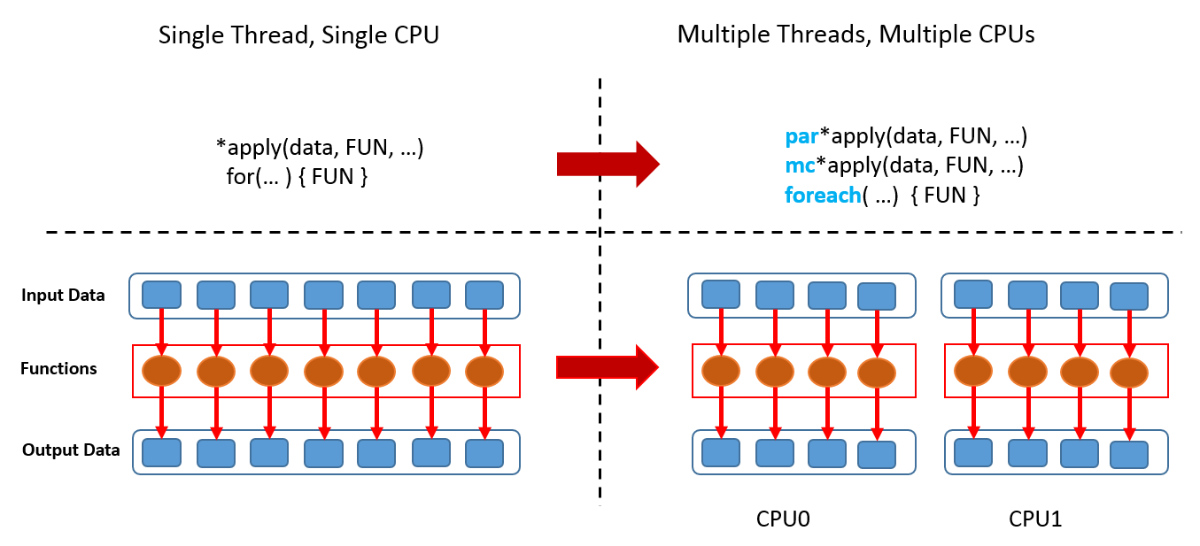

36 / 55

4. Parallelisation

"Embarrassingly parallel operations"

Source: https://bit.ly/2OX6e3e

37 / 55

4. Parallelisation

Example: parallelised bootstrapping

Remember the function cor_df() from the case study in 2. Do as Little as Possible. A faster approach, cor_df2(), is given below.

n <- 1e4
df <- data.frame(a = rnorm(n), b = rnorm(n))
cor_df2 <- function(x, n) {
  i <- sample.int(n, n, replace = T)
  cor(df$a[i], df$b[i])
}

38 / 55

cor_df2() would be even faster if df was a matrix object.

function(df, n) {
  i <- sample(1:n, n, replace = T)
  m <- df[i,]
  cor(m)[2, 1]
}

4. Parallelisation

Example: parallelised bootstrapping — ctd.

Calling cor_df2() a large number of times is time consuming.

# serial computation
s_ser <- system.time(
  r_ser <- lapply(1:1e5, function(x) cor_df2(df, n))
)
s_ser

##     
##   user  system  elapsed 
## 41.258   7.497  48.835

39 / 55

4. Parallelisation

Example: parallelised bootstrapping — ctd.

Luckily, it is straightforward to bootstrap in parallel using mclapply().

# parallel computation
s_par <- system.time(
  r_par <- mclapply(1:1e5, function(x) cor_df2(df, n), mc.cores = 8)
)
s_par

##     
##   user  system  elapsed 
## 38.343   7.995   16.343

Note that using 8 cores in my case is (only) ~5 times faster than the serial approach due to overhead.

40 / 55

4. Parallelisation

Example: too much overhead

Parallelisation may be inefficient:

system.time(mclapply(1:1e5, sqrt, mc.cores = 8))

## 
## ##   user  system elapsed 
## ##  0.107   0.110   0.062 
##

system.time(lapply(1:1e5, sqrt))

## 
## ##   user  system elapsed 
## ##  0.034   0.001   0.035 
##

This is because the cost of the individual computations is low, and additional work is needed to send the computation to the different cores and to collect the results: The overhead exceeds the time savings.

41 / 55

4. The `MonteCarlo` Package

Why is worthwhile to get used to such packages?

Running MC simulations is an everyday task in econometrics: simulations are routinely used for approximating quantities which cannot be derived analytically, e.g., finite sample properties of a test statistic.
MC simulation is also an essential tool in statistical programming because we often write functions that expect random input and/or produce random output

Testing whether the impementation is correct amounts to checking if the statistical properties of the output are as expected, using a large number of samples
Often, the effort to write the simulation exceeds the effort to implement the function by a multiple

42 / 55

4. The `MonteCarlo` Package

The MonteCarlo package streamlines the process of writing MC simulations.

Useful features are:

Simulation over a user-defined parameter grid
Automatic parallelisation using the snow package
Compilation of the results in an array. Generation of customisable LaTeX tables is possible.

The package is available on CRAN.

Development version @ https://github.com/FunWithR/MonteCarlo

43 / 55

4. The `MonteCarlo` Package

Example: Unit Root test

Consider the DGP $y_{t} = ρ y_{t - 1} + ϵ_{t}, ϵ_{t} \sim N (0, 1)$ with $y_{0} = 0$ and $ρ = 1.$ It is a well known result that the limit of the $t$ -ratio $t = \frac{\hat{ρ} - 1}{S E (\hat{ρ})}$ can be written as a functional of Wiener processes,

$t \Rightarrow \frac{[W (1)]^{2} - 1}{2 \sqrt{\int_{0}^{1} [W (r)]^{2} d r}} .$

The asymptotic distribution of $t$ is non-normal and its quantiles cannot be derived analytically.

44 / 55

4. The `MonteCarlo` Package

Example: Unit Root test — ctd.

We use the MonteCarlo package to simulate the limit distribution of $t$ .

library(MonteCarlo)

sim <- function(rho, Time) {
  Y <- matrix(NA_real_, ncol = 1, nrow = Time); Y[1,1] <- rnorm(1)
  for(t in 2:Time) { Y[t, 1] <- rho * Y[t-1, 1] + rnorm(1) }
  y <- Y[-1, , drop = FALSE]
  ylag <- Y[-Time, , drop = FALSE]
  fit <- lm.fit(ylag, y)
  rho <- fit$coefficients
  res <- fit$residuals
  sigma <- sqrt(1/(Time-2) * t(res) %*% res * 1/ (t(ylag) %*% ylag))
  return( list("t" = (rho[[1]] - 1)/sigma) )
}

45 / 55

4. The `MonteCarlo` Package

Example: Unit Root test — ctd.

# setup list of parameters
params <- list("rho" = 1, 
               "Time" = 1000)
# run parallelised MC simulation over parameter grid
r <- MonteCarlo(
  sim,
  nrep = 50000,
  param_list = params, 
  ncpus = parallel::detectCores()
)

We transform the simulated test statistics to a vector.

t_sim <- apply(r$result$t, 3, c)

46 / 55

4. The `MonteCarlo` Package

Example: Unit Root test — ctd.

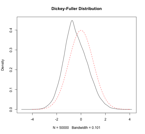
Estimates of the finite sample quantiles are close to the quantiles of the corresponding asymptotic Dickey-Fuller distribution

quantile(t_sim, c(0.05, 0.1, 0.5, 0.9, 0.95))

##         5%        10%        50%        90%        95% 
## -1.9472738 -1.6124977 -0.5044926  0.8846489  1.2702348

fUnitRoots::qunitroot(c(0.05, 0.1, 0.5, 0.9, 0.95), trend = "nc")

## [1] -1.9408468 -1.6167526 -0.4999276  0.8877673  1.2836012

We compare with the Gaussian distribution.

plot(density(t_sim), main = "Dickey-Fuller Distribution")
curve(dnorm(x), from = -4, to = 4, add = T, lty = 2, col = "red")

47 / 55

4. The `MonteCarlo` Package

Example: Unit Root test — ctd.

48 / 55

4. The `MonteCarlo` Package

It is a great benefit to work with the package if you want to run the simulation for several parameter combinations.

Example: Power of DF-Test

We write a simple wrapper for sim() which returns a logical value for rejection at 5% using the asymptotic critical value.

# asymptotic 5% critical value of the corresponding DF-distribution
crit <- fUnitRoots::qunitroot(0.05, trend = "nc")
# rejection?
sim_pow <- function(rho, Time) {
  return(
   list("t" = sim(rho, Time)[[1]] < crit)   
  )
}

49 / 55

4. The `MonteCarlo` Package

Example: Power of DF-Test — ctd.

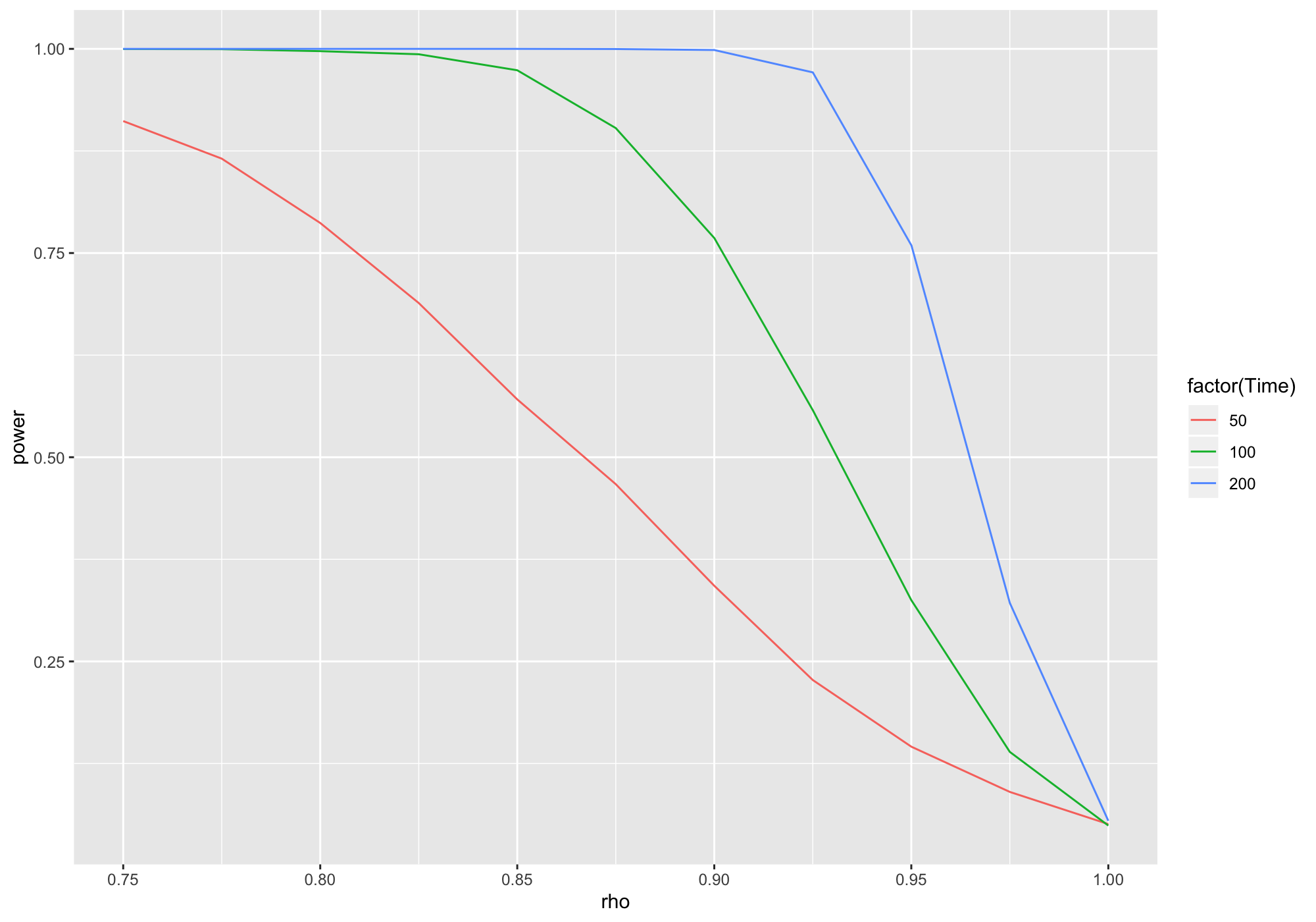
We consider all combination for a sequence of alternatives and three different sample sizes.

# setup list of parameters (yielding 33 parameter constellations)
params <- list("rho" = seq(0.75, 1, 0.025), 
               "Time" = c(50, 100, 200))
# run parallelised MC simulation over parameter grid
r <- MonteCarlo(
  sim_pow,
  nrep = 5000,
  param_list = params, 
  ncpus = parallel::detectCores())

50 / 55

4. The `MonteCarlo` Package

Example: Power of DF-Test — ctd.

Content of a MonteCarlo object is easily transformed and visualised using tidyverse functions.

library(dplyr)
library(ggplot2)
tbl <- r %>% MakeFrame() %>% tbl_df() %>% 
  group_by(rho, Time) %>% summarise(power = mean(t))
ggplot(tbl) + 
  geom_line(aes(x = rho, y = power, col = factor(Time)))

51 / 55

4. The `MonteCarlo` Package

Example: Power of DF-Test — ctd.

52 / 55

4. The `MonteCarlo` Package

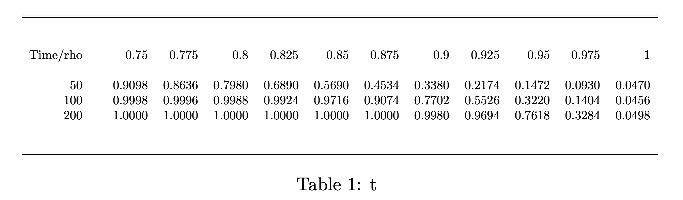
Example: Power of DF-Test — ctd.

Conversion of the results into a $L A T E X$ table is particularly useful.

# generate LaTeX table from simulation results
MakeTable(r, rows = "Time", "rho")

53 / 55

References

Gillespie, C. and Lovelace (2016), R. Efficient R Programming. O'Reilly Media.

Peng, Roger D. (2016). R Programming for Data Science. The bookdown Archive.

Wickham, H. (2019). Advanced R. 2nd Edition. Taylor & Francis, CRC Press.

54 / 55

Thank You!

55 / 55

Improving Performance

# packages needed library(tidyverse) # for bench package library(parallel) library(MonteCarlo)

We should forget about small efficiencies, say about 97% of the time: premature optimisation is the root of all evil. Yet we should not pass up our opportunities in that critical 3%. A good programmer will not be lulled into complacency by such reasoning, he will be wise to look carefully at the critical code; but only after that code has been identified. — Donald Knuth

↑, ←, Pg Up, k	Go to previous slide
↓, →, Pg Dn, Space, j	Go to next slide
Home	Go to first slide
End	Go to last slide
Number + Return	Go to specific slide
b / m / f	Toggle blackout / mirrored / fullscreen mode
c	Clone slideshow
p	Toggle presenter mode
t	Restart the presentation timer
?, h	Toggle this help

Advanced R for Econometricians

Improving Performance

Martin C. Arnold

Improving Performance

Improving Performance — Overview

1. Look for Existing Solutions

Improving Performance — Golden Rule

2. Do as Little as Possible

Exercise: coercion of inputs / robustness checks

2. Do as Little as Possible

Exercise: coercion of inputs / robustness checks — ctd.

2. Do as Little as Possible

Exercise: searching a vector

2. Do as Little as Possible

Exercise: Linear Regression — computation of SE(ˆβ)SE(β^)

2. Do as Little as Possible

Example: method dispatch takes time

2. Do as Little as Possible

Example: primitives are faster

2. Do as Little as Possible — Exercises

2. Do as Little as Possible — Case Study

3. Vectorise your code

3. Vectorise your code

3. Vectorise your code

Example: vector addition

3. Vectorise your code

3. Vectorise your code

Example: scalar vs. vectorised computation of euclidean norm

3. Vectorise your code

Example: scalar vs. vectorised computation of euclidean norm

3. Vectorise your code — Some Principles

3. Vectorise your code

3. Vectorise your code

Example: avoid growing objects

3. Vectorise your code

Example: good and bad for() loops

3. Vectorise your code

Example: good and bad for() loops

3. Vectorise your code

Example: good and bad for() loops

3. Vectorise your code

Example: for() vs. apply()

3. Vectorise your code

Example: for() vs. apply() — ctd.

3. Vectorise your code — Exercises

3. Vectorise your code — Case Study

3. Vectorise your code — Case Study

4. Parallelisation — FAQs

4. Parallelisation — FAQs

4. Parallelisation — the parallel package

4. Parallelisation - parallel::mclapply()

Example: send them cores to sleep (on MacOS)

4. Parallelisation - parallel::mclapply()

Example: send them cores to sleep (on MacOS) — ctd.

4. Parallelisation - parallel::mclapply()

Example: send them cores to sleep (Windows)

4. Parallelisation

4. Parallelisation

Example: parallelised bootstrapping

4. Parallelisation

Example: parallelised bootstrapping — ctd.

4. Parallelisation

Example: parallelised bootstrapping — ctd.

4. Parallelisation

Example: too much overhead

4. The MonteCarlo Package

4. The MonteCarlo Package

4. The MonteCarlo Package

Example: Unit Root test

4. The MonteCarlo Package

Example: Unit Root test — ctd.

4. The MonteCarlo Package

Example: Unit Root test — ctd.

4. The MonteCarlo Package

Example: Unit Root test — ctd.

4. The MonteCarlo Package

Example: Unit Root test — ctd.

4. The MonteCarlo Package

Example: Power of DF-Test

4. The MonteCarlo Package

Exercise: Linear Regression — computation of $S E (\hat{β})$

Example: good and bad `for()` loops

Example: good and bad `for()` loops

Example: good and bad `for()` loops

Example: `for()` vs. `apply()`

Example: `for()` vs. `apply()` — ctd.

4. Parallelisation — the `parallel` package

4. Parallelisation - `parallel::mclapply()`

4. Parallelisation - `parallel::mclapply()`

4. Parallelisation - `parallel::mclapply()`

4. The `MonteCarlo` Package

4. The `MonteCarlo` Package

4. The `MonteCarlo` Package

4. The `MonteCarlo` Package

4. The `MonteCarlo` Package

4. The `MonteCarlo` Package

4. The `MonteCarlo` Package

4. The `MonteCarlo` Package

4. The `MonteCarlo` Package

4. The `MonteCarlo` Package

4. The `MonteCarlo` Package

4. The `MonteCarlo` Package